Data access and acquisition

Getting your data

Your options include:

copying data directly from the network drive where it’s stored - see note below
using SFTP - see note below
using Globus Connect - see note below

The beamline staff typically use the first option.

Caution

The use of USB drives to transfer data is convenient, but poses a security risk. Get permission from your local contact.

To speed-up post-beamtime data analysis and reduce the amount of raw data to be taken home, we recommend:

using the User Data Analysis workstation in the measurement hutch,
creating one or multiple Igor project files and saving them locally,
importing the good measurement files into the Igor project file(s) and working with them (e.g. performing drift correction, extracting spectra using z-profiles, etc.),
using folders within the project file(s) to organize the data, and the notebooks within Igor to perform logging,
copying the Igor project files to your PC and/or hard drive(s) at the end of your beamtime, and
backing up your Igor project file(s) to the processed sub-folder, under your proposal folder.

Copying data directly from the network drive

Connect to the maxiv_user Wi-Fi network (which requires your DUO username and password).

Map/mount the network drive folder relevant for your proposal. On a Windows computer, you would mount \offline-2.maxlab.lu.se\offline-visitors\maxpeem\12345678

where 12345678 is your 8 digit proposal number. Use the username MAXLAB\xxxx where xxxx is your DUO username, and your DUO password.

Note that practical data transfer speeds are ~5 MB/second.

SFTP

See the MAX IV SFTP webpage.

Globus Connect

See the MAX IV Globus Connect webpage

To-do before measurement

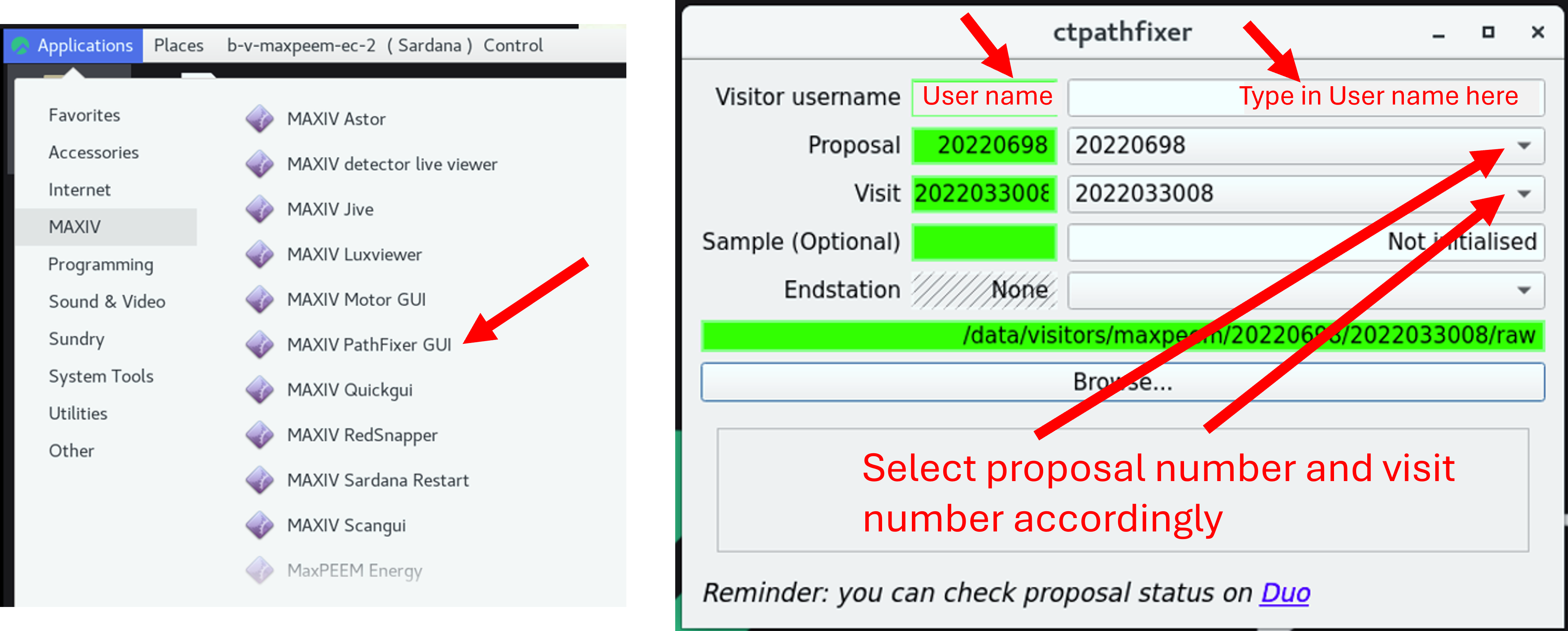
Storage location of data (check before starting the sequence)

Edit mode – Storage – Change the file name accordingly if wants to, e.g. date.

File path will be automatically updated to raw folder once finish ctpathfixer.

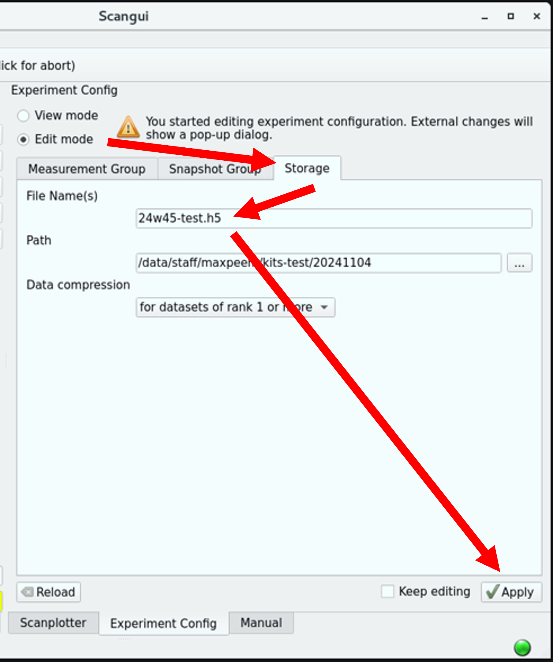
Note

The generated .h5 file (dated format) contains valuable information, such as the beam intensity measured with the gold mesh for normalization.
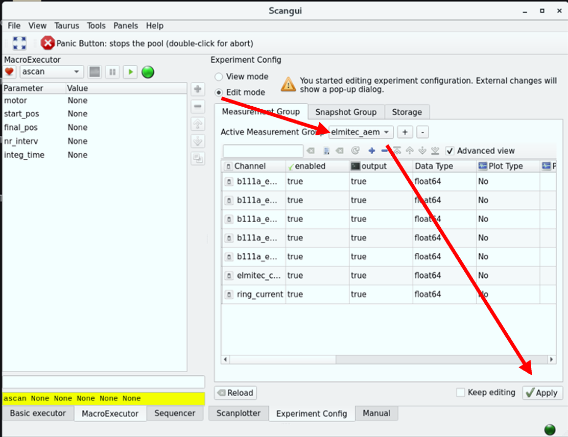
To review the collected data: Check the Measurement Group and Snapshot Group in scangui.

Active measurement Group: elmitec_aem (default)

Edit mode – select elmitec_chan – apply

Beamline alignment

Control panel (MaxPEEM energy)

Application – MAXIV – MaxPEEM energy (during measurements, use the standard mode only) Extended view with Expert mode is used for aligning M1_Pitch.

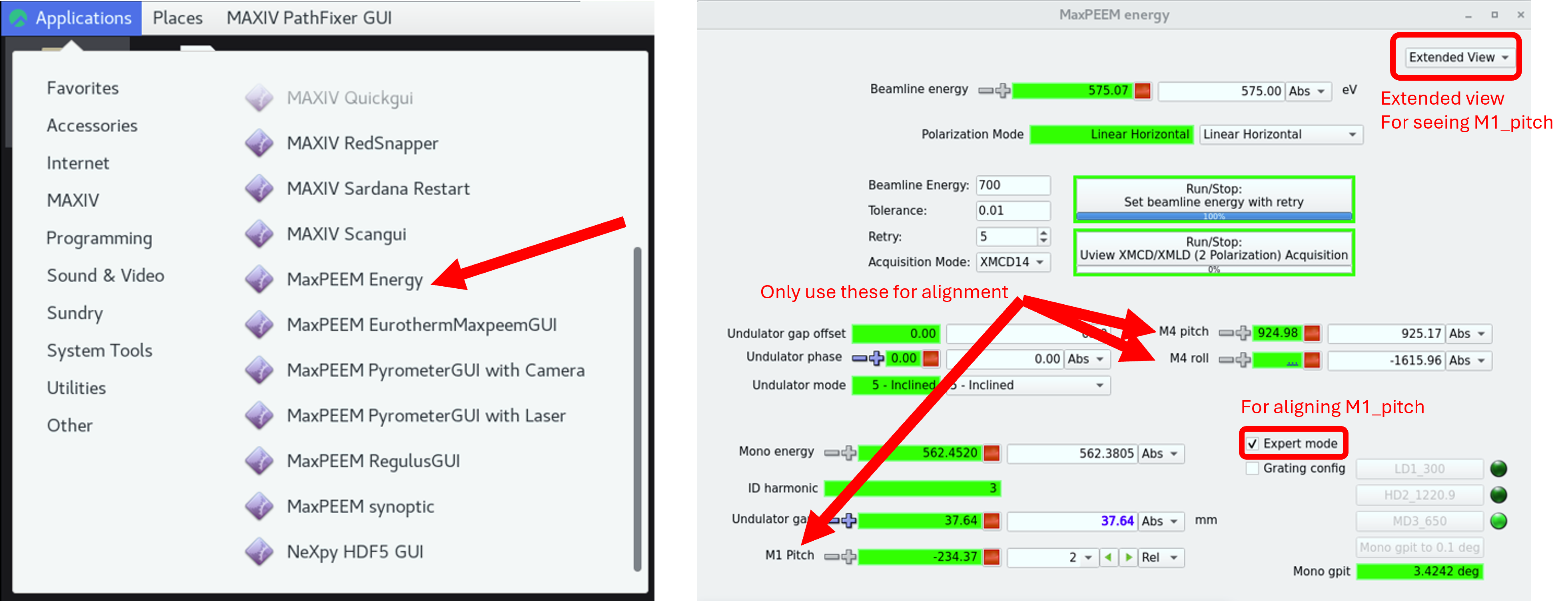
Maximize beam intensity using M1_pitch, step=2
- One can use the photodiode in beam path (value=78 means photodiode is inserted).
Localize beam at center of image and make it uniform using M4_pitch (step = 2) and M4_roll (step = 10)

If defocusing is needed, use M4_yaw (step = 10) and then correct beam position with M4_pitch and M4_roll.

Note

During beamline alignment, field of view can be enlarged with decreasing P3 value, instead of change FoV setting.

When Beam dump unfortunately happened: valves automatically closed and beam current was not 500 mA. Check the chat panel for updates.

Open valves in front end

Public website for machine status

To open: V1, BS-01, HA-01

To close: HA-01, BS-01, V1

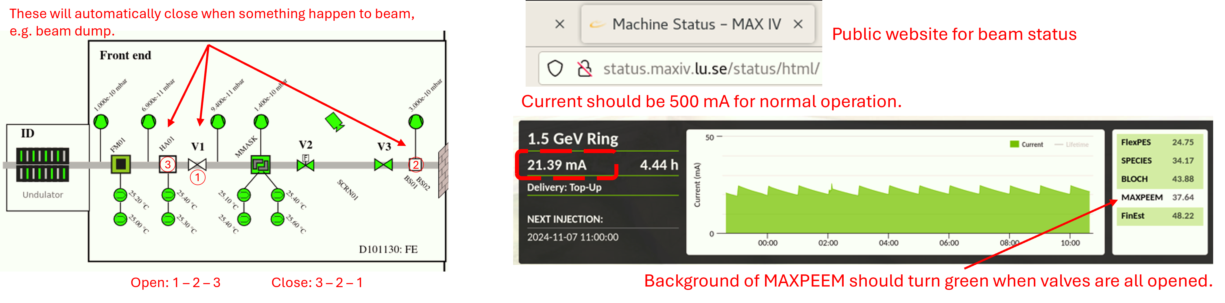
HA-01 and BS01 are used for blocking beam, and V1 is used for isolating the vacuum of storage ring.
The beam is opened or closed in this order to prevent direct illumination of beam on V1, which is metal and might melt under illumination.

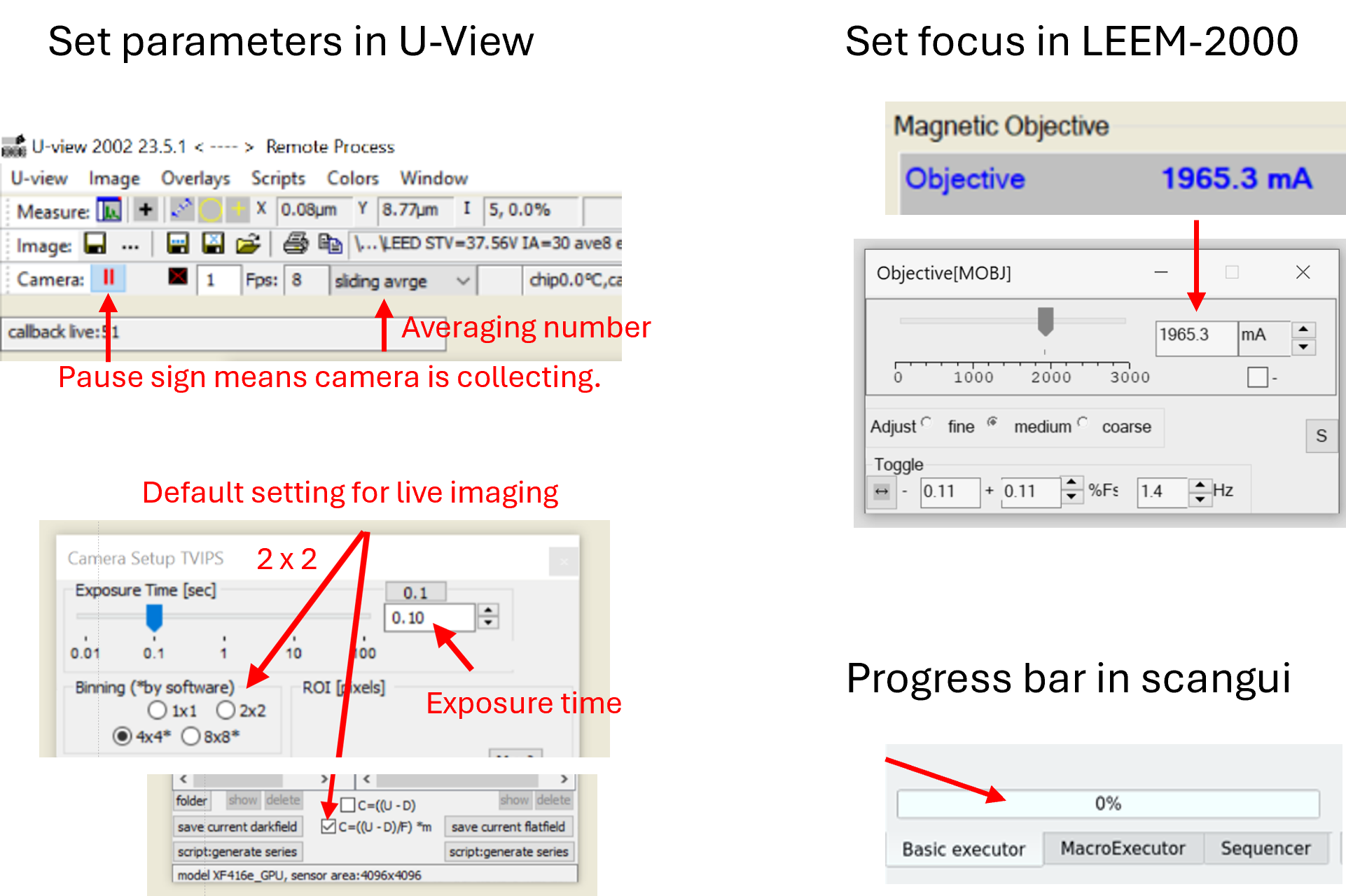
U-view software interface with frequently used function

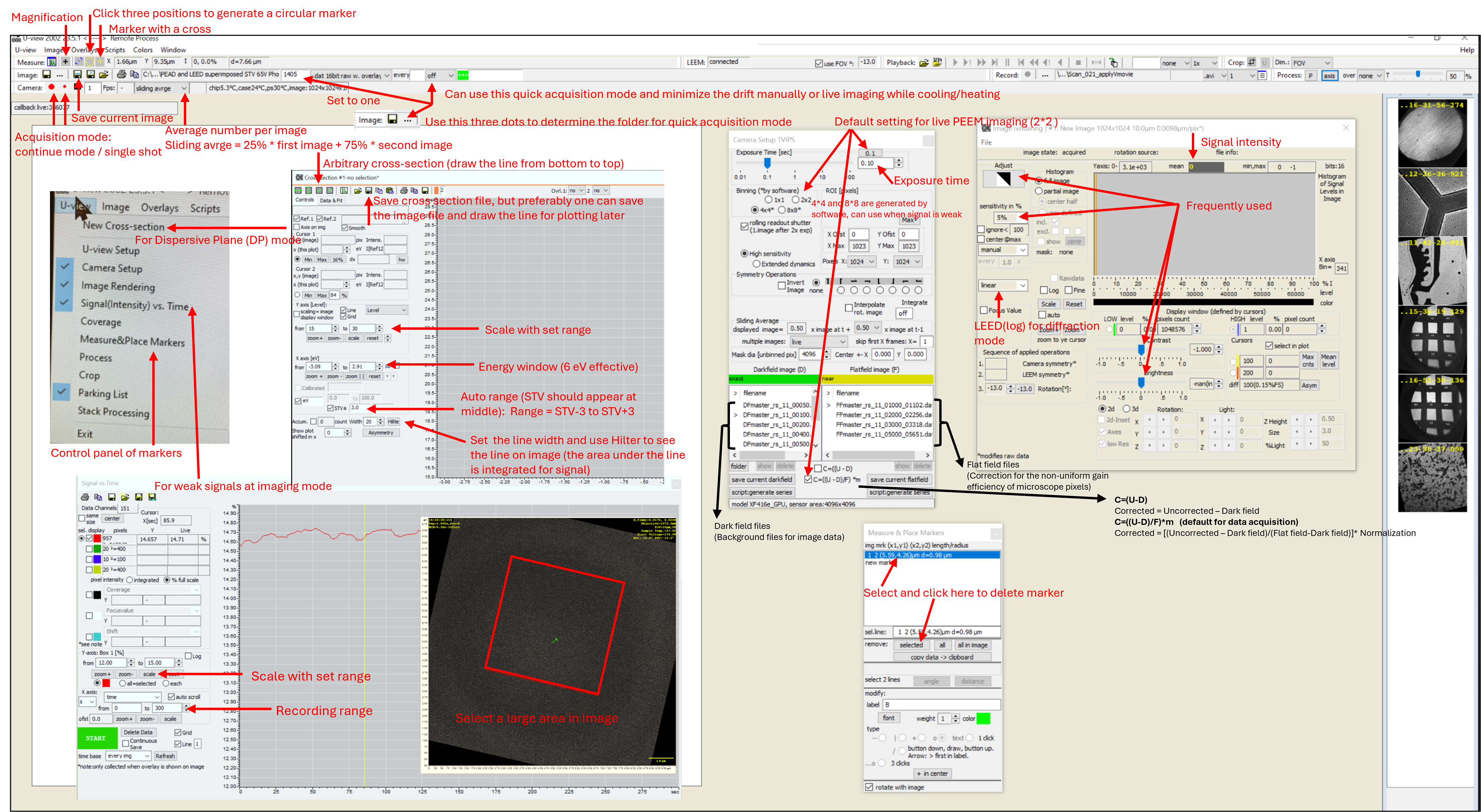
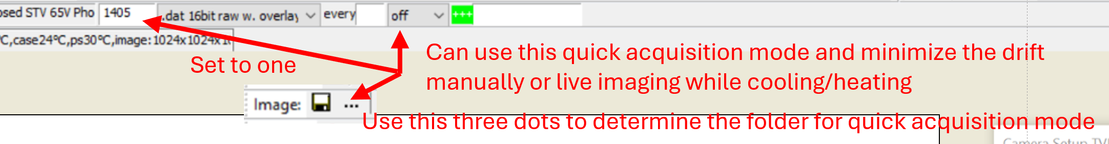
Continuous quick acquisition

This function is useful when the drift is severe or collecting live images while cooling or heating.

Determine the folder for saving the image sequences with the three dots in Image channel.
(Optional) Set the start file number to 1.
Set up suitable exposure time and averaging times.
Set up suitable collection way, for example ‘every 5 sec’ means the image will be saved every 5 seconds, with the set exposure time and averaging times.
Turn on live mode of micrscope. (Click on red big circle)

Remember to turn off this function after finish using it.

µ-XPS (DP mode)

Caution

Since the energy slit is not in the path, be careful about setting Start Voltage!

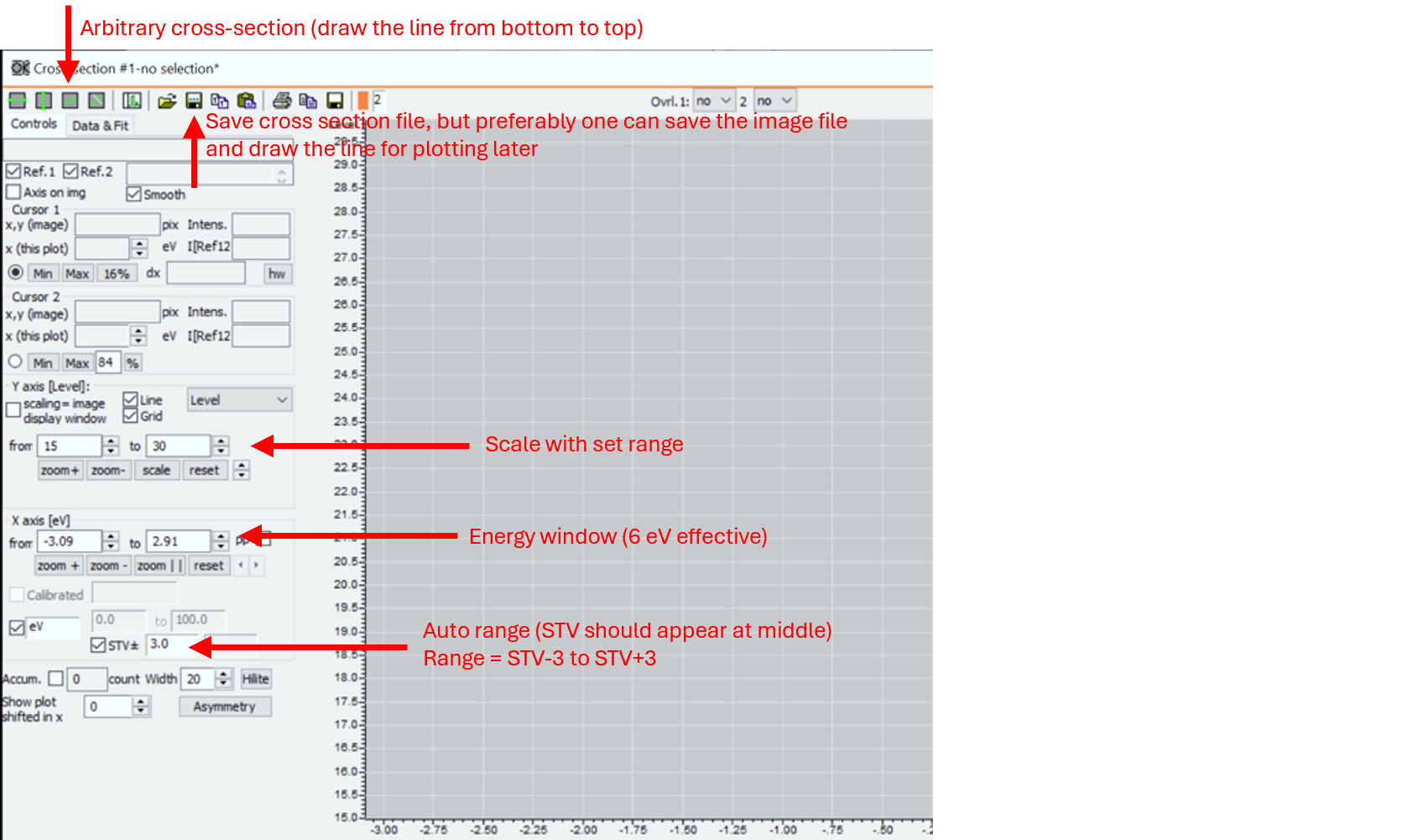
U-view – Arbitrary cross-section – draw a line from bottom to top – (if available) adjust start voltage to see Au doublet with energy difference ~3.6 eV *Save the spectrum as reference!

Useful values: Available energy window: ~ 6 eV; Work function: ~ 4.85 eV

Energy window is limited to 6 eV (effective range) but the energy resolution (~ 0.2 eV, depends on SAA, can be better) is better than XPS in XPEEM mode (~ 0.5 eV, depends on step setting and signal intensity).
Steps for determining the measurement parameters are same as XPS in XPEEM mode.
Click on the box for eV and STV±3, so that the set STV should appear at middle of energy range.
Click on Hilte, which can change the line width with maximum as 40. Intensity is integrated from the area marked by the line, so increasing line width can provide strong signal.

XPEEM (scan start voltage)

Moveable in scan = leem_start_voltage

Check the coefficient plot of desired element, e.g., Pt. Determine the target orbit, e.g. Pt 4f based on the plot.
Determine the photon energy (e.g., hv = 250 eV) based on the coefficient plot and beamline energy profile, i.e. where it emits most and where the beamline intensity is highest.
Check the binding energy of target orbit, e.g., Pt 4f has binding energies as 74.5 and 71.2 eV.
Calculate the corresponding start voltage, e.g., as 170.5 (250-5-74.5) and 173.8 (250-5-71.2) V.
Set up scangui or script or IPython to scan the range.

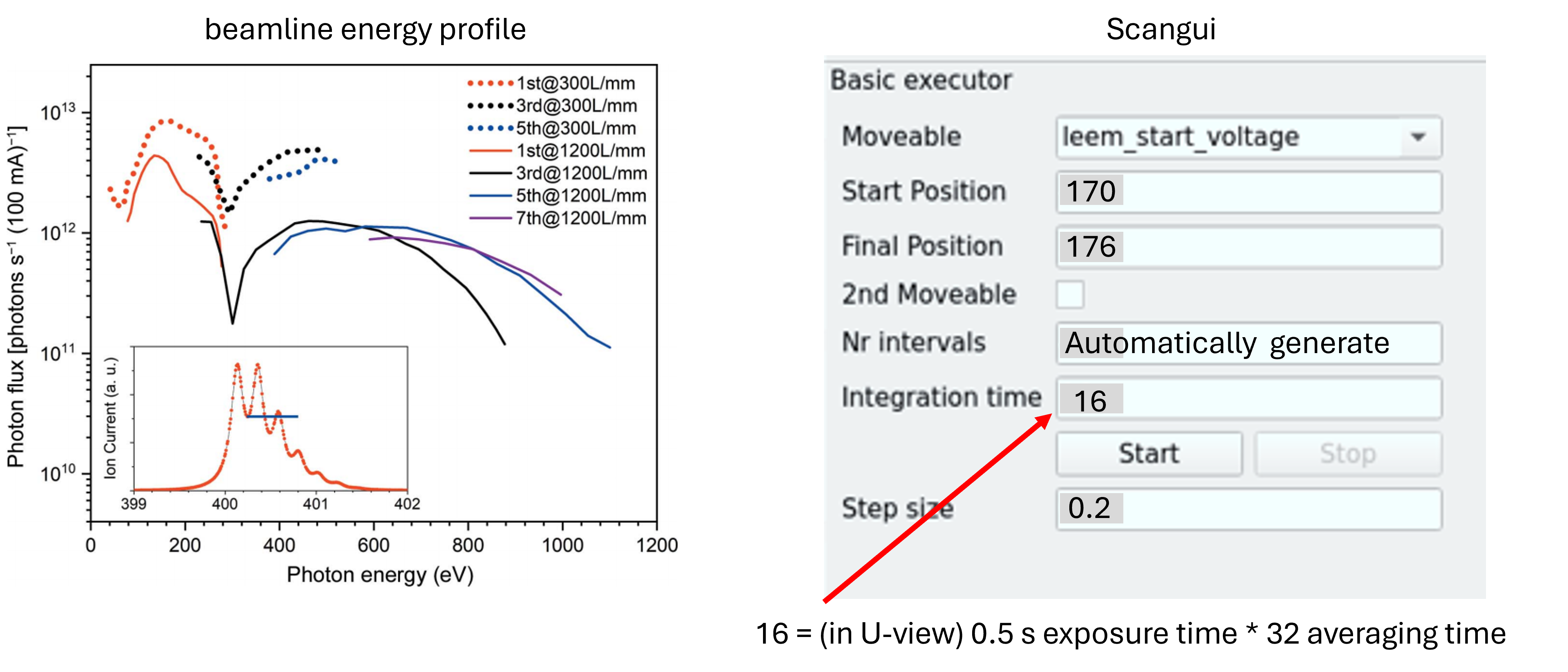
If the signal is too weak, one can use the ‘IntensityVsTime’ in LEEM2000 software, with selecting a large area on sample. Change the start voltage slowly in the calculated range and observe the change in intensity. Write down the values for determining the scan range later. In addition, the written down values can be compared to the calculated values as checking. Check U-view software interface for details.

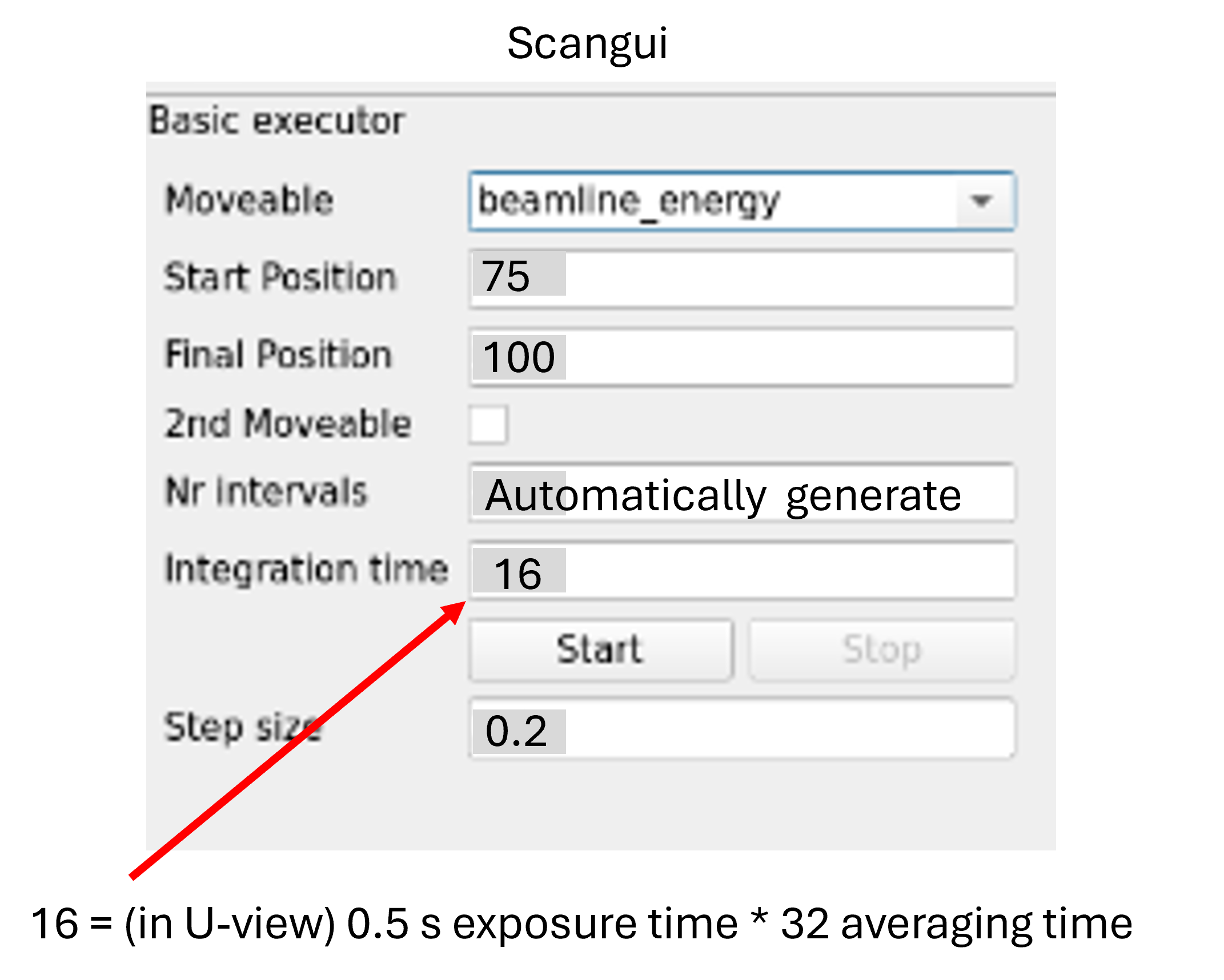
XAS

Moveable in scan = beamline_energy

Set the start voltage to a higher value.
Set photon energy accordingly, e.g. 75 eV for Al as scan range (written on the paper on wall behind the screen) is Al 75 to 100 eV. The table can be found at end of this page or in online source.
Reduce the start voltage to identify the secondary electron peak, i.e., aiming to maximize the image intensity.
Set up scangui or script or ipython to scan the range.

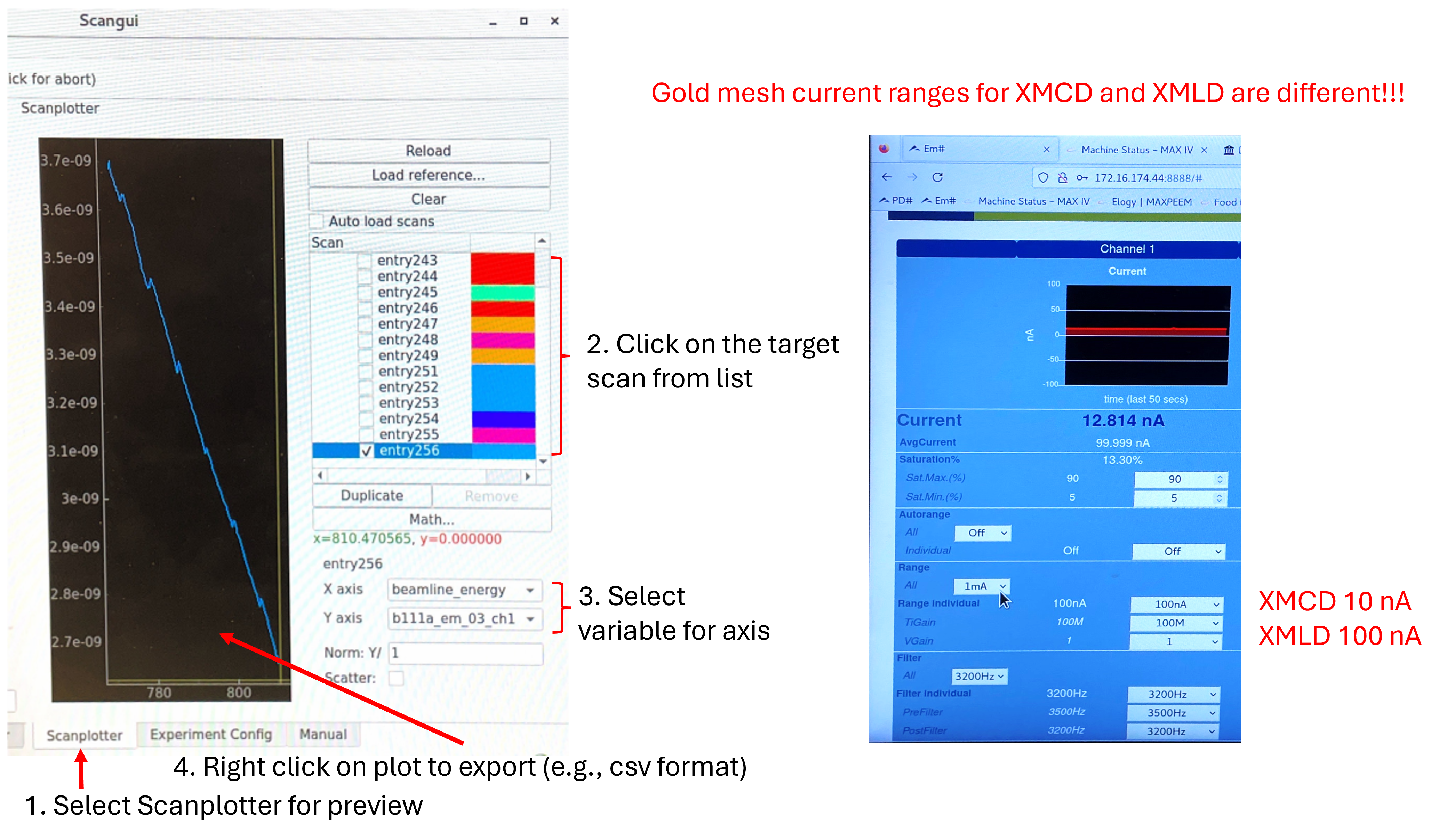
XMCD-/XMLD-PEEM

Note

The ranges of gold mesh current (measured for normalization) are different for XMCD and XMLD as the beamline intensity differs significantly in these two modes. Check the interface here.

Collect individual image for XMCD (circular left, circular right)

(if haven’t done before) Save LEEM alignment setting, electron gun OFF, open x-ray valve and check beam alignment.

(Optional) One can start with XAS to determine the photon energy, as well as checking if sample is oxidized.
Change to the desired photon energy, change the undulator mode to 2.Helical and change the polarization mode to circular left 14 or circular right 14 which are frequently used.
Set up U-view camera parameters, exposure time and averaging time, collect the image data and save it.

The Rel function, which adjusts the beamline energy relatively, can be used with a step size of 0.2 to test the suitability of the selected energy while observing the image.
Set gold mesh current range to 10 nA.

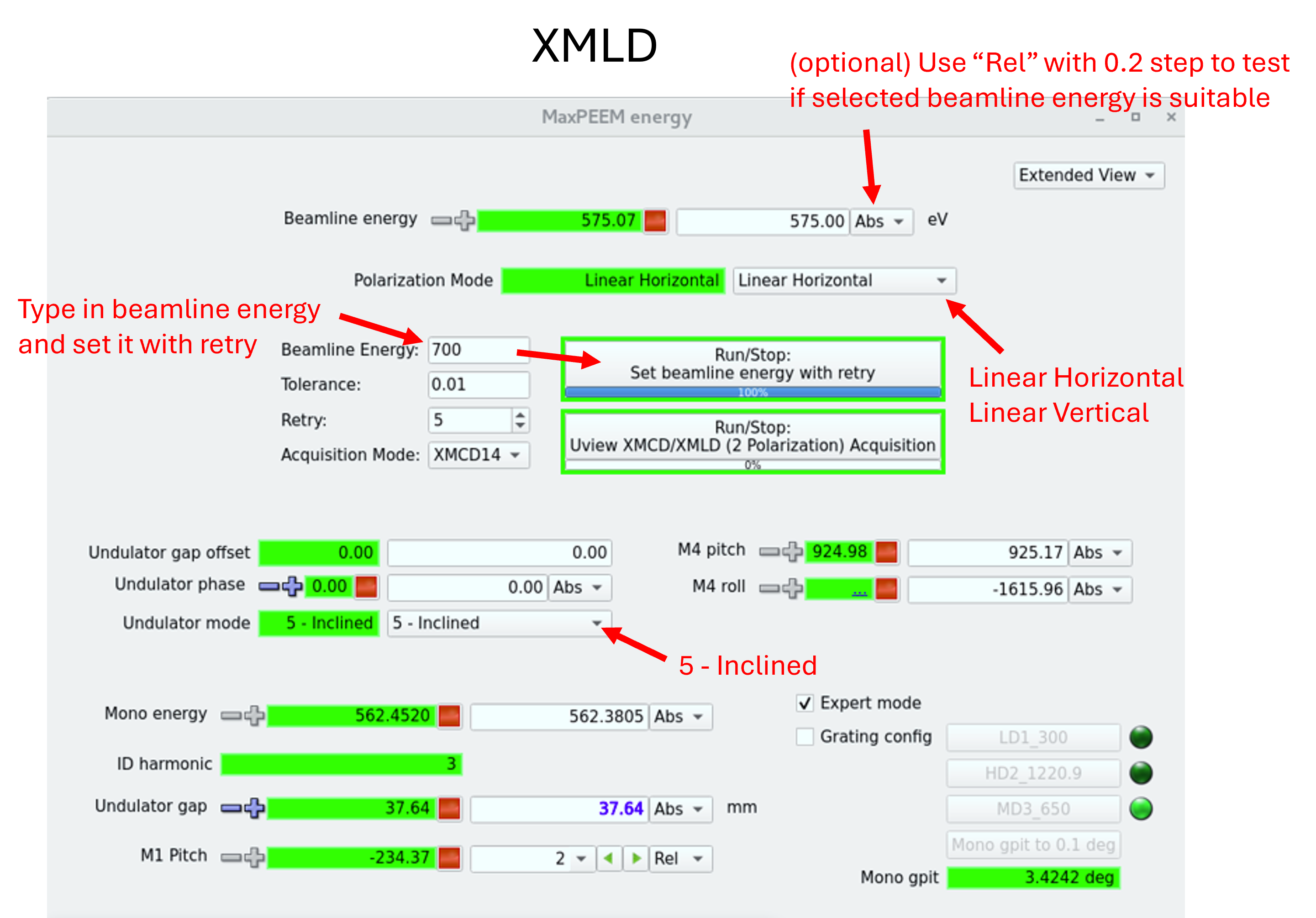
Collect individual image for XMLD (linear horizontal, linear vertical)

(if haven’t done before) Save LEEM alignment setting, electron gun OFF, open x-ray valve and check beam alignment.

(Optional) One can start with XAS to determine the photon energy, as well as checking if sample is oxidized.
Change to the desired photon energy, change the undulator mode to 5 - Inclined and change the polarization mode to linear horizontal or linear vertical which are frequently used.
Set up U-view camera parameters, exposure time and averaging time, collect the image data and save it.

The Rel function, which adjusts the beamline energy relatively, can be used with a step size of 0.2 to test the suitability of the selected energy while observing the image.
Set gold mesh current range to 100 nA.

Scangui

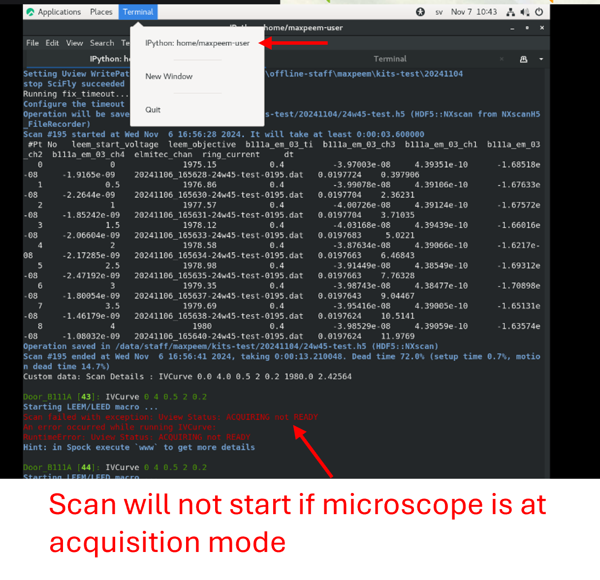
Caution

Camera must not be in collecting mode when starting scan. During acquisition (before progress reaches 100%), don’t hit any part of setup which will cause vibrations and blur the image, e.g. transfer arm, concrete base of setup, etc.

Check the storage location of data files. Filename can be changed.
Parameters need to be matched between camera setting and scangui setting. For example, the integration is set as 80. In U-view (microscope software), the image is collected with ‘average 16’ and exposure time is 5. So that parameters are matched as 80=16x5.

Note

If beamline energy is changed in sequencer, e.g. XPEEM of Au 4f (E_ph = 250 eV) and Au VB (E_ph = 70 eV), remember to add executor to change objective lens value for each scan. Check equation and examples.

Sequencers

Two commonly used ways to set up the sequencer:

Basic executor: normally only one moveable is used, but the second one can be activated if needed
MacroExecutor: more customizable functions can be used, e.g. ascan, IVCurve, mesh, mv, uview_acquisition, uview_ascan, uview_xmcd_xmld_acquisition, etc. Move moveables can be added from panel.

Select the moveable, type in start and final positions, type in integration time (averaging number*exposure time) and step size. The Nr internals will be calculated automatically based on the set parameters.
Check the storage and change filename if needed.

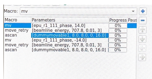
Set up Macroexecutor

Check the saved macros in the commissioning folder to see if they meet your requirements. The following outlines the logic for building a macro for XMCD measurements with Circular Left (CL) and Circular Right (CR) polarization:

Set Polarization to Circular Left (CL):
mv - Change phase to 14.
Set Energy with Retry:
move_retry - Target beamline energy to 707.8 eV.
- Allowable deviation: ±0.01 eV
- Maximum retries: 3
Collect Image:
ascan - Capture one image with:
- integ_time=16 (0.5 s × 32 averaging)
- start_pos=final_pos (e.g., 8)
- nr_interv=0
Set Polarization to Circular Right (CR):
mv - Change phase to -14.
Repeat Energy Retry:
move_retry - Same settings as above.
Capture Second Image:
ascan - Use the same settings as in Step 3.

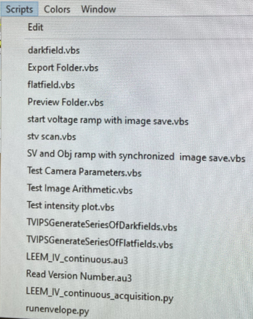
Scripts (Might be updated)

*Data can only be written into ‘This PC’ instead of online user folder.

Ipython

For users who prefer to scan via Terminal: Type in parameters as if in scangui

Naming data files

Naming of data file:

Mode name (XPEEM/LEEM/DP/ARPES/LEED) + Sample name + Element + Orbit + Photon energy + Start Voltage + IA value (if used) + SAA value (if used) + CA value (if used) + Slit value (if used)

Naming of data folder for sequence: Mode name (XPS/XAS) + Sample name + Element + Orbit + Photon energy (or range) + Start Voltage (or range) + Integration time (averaging number + exposure time in U-view software) + Step size + IA value (if used) + SAA value (if used) + CA value (if used) + Slit value (if used)

If sample has been moved more than hundreds of µm (1-2 mm) at any direction, alignment needs (has) to be double checked.
Example for Values needed before starting sequences: Photon energy, Start Voltage, Slit and Apertures, Averaging time and Exposure time, Value of Objective lens for each sequence

Examples for mapping ranges

Work function of setup ~ 4.85eV

Remember to find the focus (Value of Objective lens) for each sequence:

When KE = 0, \(f = f_{0}\)

When KE ≠ 0, \(f = f_{0} + α * \sqrt{KE}, α = 3.576\)

The ranges advised below are just examples. If uncertain, please consult with beamline scientist.

XAS measurement by scanning beamline energy

Element (Edge)	Range (eV)
Mn (L)	635-660
Fe (L)	703-730
Cr (L)	570-595
Ni (L)	847-880
Co (L)	770-810
O (K)	528-553
Ti (L)	458-479
Ca (L)	345-360
N (K)	395-440
S (L)	150-190?
Al (L)	75-100
Si (L)	100-125
Zn (M)	325-360

Technique	E_Ph (eV)	STV	Exposure	Average	Step	Objective Value	BE (eV)	Notes
XPS (XPEEM)
Au 4f	250	155.8 to 156.4	5	16	0.2	1867	84
Au VB (5d)	70	55 to 68 (65)	2	16	0.2	1857
Au WF	70	-3 to 4	0.1	16	0.1	1835
PED (ARPES)
Au + Graphene	70	63 to 66.5 (65)	5	8	0.1
PES (DP mode)
Si 2p	150	44						PES Si 2p SAA=50 µm CA=30 µm hν=150 eV STV=44 V
Si 2p	200	94						Add 50 eV in photon energy and start voltage
Au 4f (doublet)	200	109						Use the energy difference of doublet (3.6 eV) to calibrate pixel
Au VB (+SiC, C)	200	194
C 1s	350	61.5
VB	100	94						Beam at 100 eV is stronger than at 200 eV; measure with stronger signals. Same spectrum with better signal-to-noise ratio. 100=200-100, 94=194-100.

Data access and acquisition

Getting your data

Copying data directly from the network drive

SFTP

Globus Connect

To-do before measurement

User-related information (type in before measurements)

Storage location of data (check before starting the sequence)

Gold mesh related info (02/04/2025)

Active measurement Group: elmitec_aem (default)

Beamline alignment

Control panel (MaxPEEM energy)

Open valves in front end

U-view software interface with frequently used function

Continuous quick acquisition

µ-XPS (DP mode)

XPEEM (scan start voltage)

XAS

XMCD-/XMLD-PEEM

Collect individual image for XMCD (circular left, circular right)

Collect individual image for XMLD (linear horizontal, linear vertical)

Scangui

Sequencers

Set up Macroexecutor

Scripts (Might be updated)

Ipython

Naming data files

Examples for mapping ranges

XAS measurement by scanning beamline energy